In the previous article we have seen how to use Eclipse Deeplearning4j for building, training and testing a simple and classic MLP (Multi Layer Perceptron) neural network.
As a dataset we used the “hello world” example of deep learning, that is the MNIST: a dataset of 70,000 b/w images of 28×28 pixels, representing handwritten 0-9 digits.
Now we will explore a different architecture known as Convolutional Neural Network (CNN), which is very powerful, particularly when dealing with image classification tasks. After having explained how this network works and why it is so efficient, then we will take our previous MLP example, just change the first block of code (the network building part) and test it.
As we have seen in the first article of this series, in a classic Multi Layer Perceptron (MLP) network, each node in a layer has input connections from all the nodes in the previous layer.
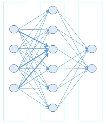
For simple networks this can be acceptable, but as soon as the number of node is growing the total number of connections will grow exponentially, which of course means much higher elaboration time in the best case, but often means no convergence in the training phase.
Moreover, in several scenarios a connection between two nodes that are spatially far from each other may be pointless. Think about a picture for instance: in most cases (e.g. object recognition) it is meaningful to analyze pixels that are close to each other: are they similar? are they part of the same object? etc…
So what are Convolutional Neural Networks? How they can help?
Well, to begin with, using CNN allows to leave unaltered the bi-dimensional aspect of an image.
In fact, with MLP networks, we had to “serialize” all the rows of pixels of a given image in order to obtain a one-dimension array of pixels
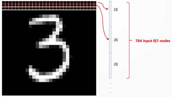
which looks a bit innatural, even if at the end it works.
Instead CNN are designed to “understand” the bi-dimensional structure of an image, so that the input of the network is an array with two dimensions: the width and the height of the image.
But the most important concept about CNN is that a given node in a layer is not fully connected to all the nodes of the previous layer, but just to a group of them, which are spatially located near the target node.
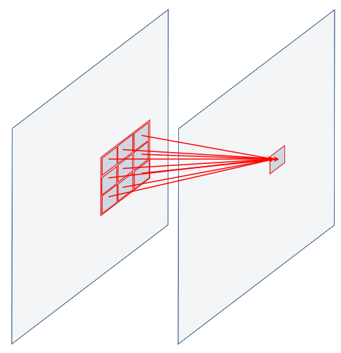
Moreover, this exact same set of connection (same weight values) is applied all over the layer, as if we were shifting and sliding this connections group step by step over all the image
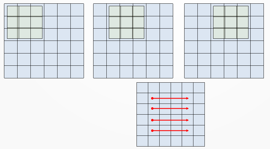
Applying a set of weights to a group of nodes means nothing less than performing a pixel-per-pixel product and an overall sum over the two matrix.
This group of connections acts therefore as a filter! Not so clear? Let’s clarify this concept with an example.
Let’s say we want to detect a top-right corner on an image. In the following figure you can see the image represented by a 6×6 pixel image (light blue for off-pixels, darker blue for on-pixels).
Imagine to overlap a 3×3 pixel filter (light orange for on-pixels of the corner detection filter).
As we slide the filter over the image we perform a pixel-per-pixel product and an overall sum (this is the Convolution operation); this operation leads to a high value when the filter pattern overlaps the portion of the image that contains a similar pattern, while it has lower values elsewhere.
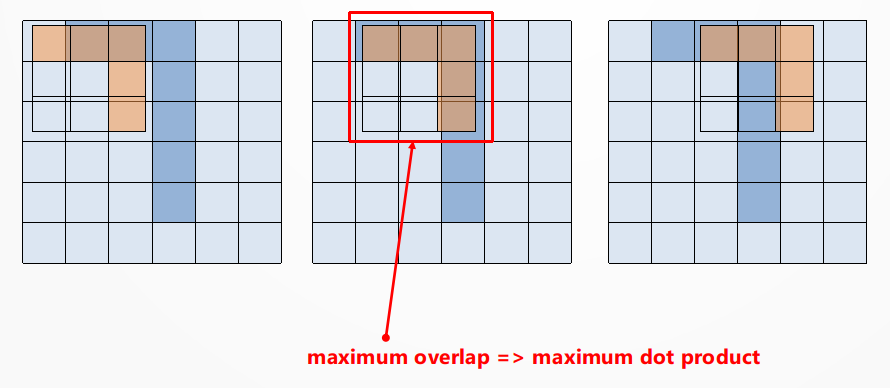
The idea of sliding the filter is just a way to explain the principle of the convolutional approach: indeed the filter is applied simultaneously to all the regions, but this doesn’t change the result.
Using this approach the number of weights between two consecutive layers is much less than in MLP network, at least for a given filter. Take for instance the example in the previous article: there we had 28×28=784 nodes in the input layer and 1000 in the hidden layer; therefore the number of weights between the two layers was 728,000.
Here, with the convolutional filter above we just have 3×3=9 weights!
Of course, in order to detect complex shapes or patterns, one filter is not enough. So we can choose to use a number of filters, each one focused on a particular feature to be detected.
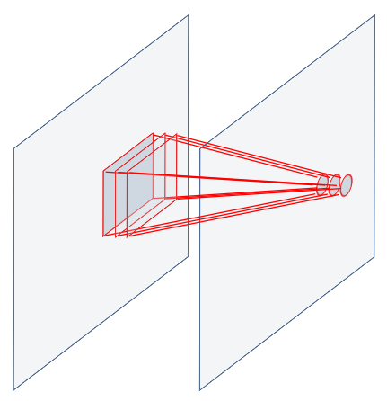
But how should we design each filter? Should we design filters for corners, vertical or horizontal lines, curves?
Well, the good news is that we don’t have to design them! We only have to choose how many they should be and their structure (e.g. 3×3, 5×5, …), along with other parameters about how to apply them.
The content of the filters (that is the feature they detect) will be the result of the training process: so the filters will auto organize themselves accordingly with the dataset and the training phase!
Typically, in a CNN, each convolutional layer is followed by a Subsampling (or Pooling) layer. What does it exactly? It reduces the dimensions of the layer itself. Let’s say we have a 2×2 subsampling layer: this means that in the previous layer each 2×2 group of adjacent cells are evaluated and a single value is calculated from them. This evaluation may be the sum (or the average) of the four cell values, like in the following figure

Therefore in case of a 2×2 subsampling layer the subsequent layer will get half of the width and height of the previous layer, so with a global one-fourth reduction.
At the end a CNN is typically composed by a number of Convolutional + Pooling layer pairs with a final outcome layer whose job is to decide which node has to be turned on from a set of N possible labels (for instance the 10 possible digits with the MNIST dataset). This final layer performs this choice using an Activation Function called SoftMax.
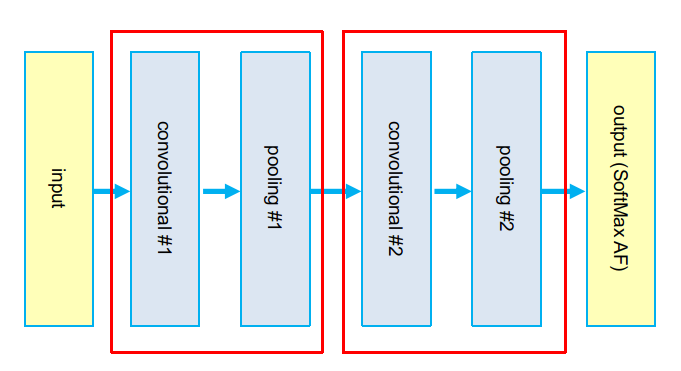
Now we can try all this with Deeplearning4j by taking the code from the previous article and change just the part where we build the network; the rest of the code can be kept exactly the same.
		int channels = 1;
		MultiLayerConfiguration conf = new NeuralNetConfiguration.Builder()
                .seed(123)
                .l2(0.0005) // ridge regression value
                .updater(new Nesterovs(0.006, 0.9))
                .weightInit(WeightInit.XAVIER)
                .list()
                .layer(new ConvolutionLayer.Builder(3, 3)
                    .nIn(channels )
                    .stride(1, 1)
                    .nOut(50)
                    .activation(Activation.RELU)
                    .build())
                .layer(new SubsamplingLayer.Builder(SubsamplingLayer.PoolingType.MAX)
                    .kernelSize(2, 2)
                    .stride(2, 2)
                    .build())
                .layer(new ConvolutionLayer.Builder(3, 3)
                    .stride(1, 1) // nIn need not specified in later layers
                    .nOut(50)
                    .activation(Activation.RELU)
                    .build())
                .layer(new SubsamplingLayer.Builder(SubsamplingLayer.PoolingType.MAX)
                    .kernelSize(2, 2)
                    .stride(2, 2)
                    .build())
                .layer(new DenseLayer.Builder().activation(Activation.RELU)
                    .nOut(500)
                    .build())
                .layer(new OutputLayer.Builder(LossFunctions.LossFunction.NEGATIVELOGLIKELIHOOD)
                    .nOut(N_OUTCOMES)
                    .activation(Activation.SOFTMAX)
                    .build())
                .setInputType(InputType.convolutionalFlat(HEIGHT, WIDTH, channels)) // InputType.convolutional for normal image
                .build();
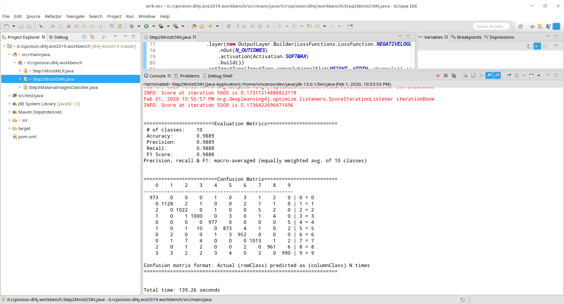
As you can see in the following figure, the results show an accuracy of nearly 99%
 |
Until now we have seen all these good principles applied on a quite simple task after all (the MNIST dataset).
Ok, so how about considering a more complex and real example?
Many of you may have heard about Kaggle: an online community of data science and machine learning experts and practitioners.
It provides courses, datasets, competitions (with prizes), forums for discussions and a lot of other resources.
Although Kaggle is somehow more Python and Keras oriented (rather than tied to Java and Deeplearning4j) when it comes to courses and discussions, it is nevertheless a highly valuable source of datasets.
Among the huge archive of datasets available from Kaggle you can find the Malaria Cell Images Dataset

This dataset contains over 27,000 images of both Malaria Infected and Uninfected cells.
Compared with MNIST here we have just two output classes instead of 10, but here we have color images much more complex than before (not simple 28×28 b/w images).
Moreover, the task of classifying them is not easy to be performed by everyone (like with MNIST images), but requires an expert in the specific medical field.
However, we can start with the code used above in this article, apply some adjustment
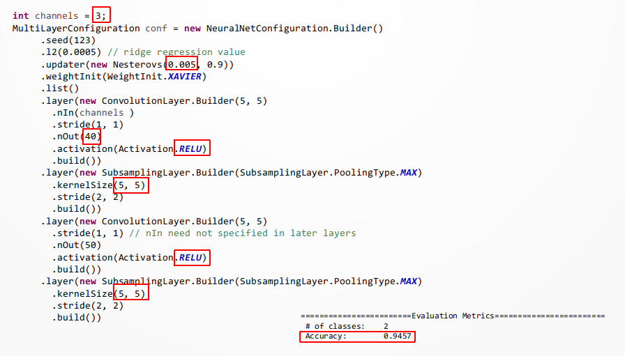
and obtain a very respectable result (94%).
Consider that the above adjustment was made just as a trial: with some more effort there is for sure extensive room for improvement.


Hello Vincenzo,
thanks for your great articles about dl4j. I (total beginner) tried to reproduce the malaria use case, but failed. Can your code about this seen online as well?
BR
Tobias
yes, sure, here
https://github.com/vincenzocaselli/dl4j-ece2019/blob/master/it.rcpvision.dl4j.ece2019.workbench/src/main/java/it/rcpvision/dl4j/workbench/Step3MalariaImagesClassifier.java
[…] published on rcp-vision.com. Reproduced here with consent of the original author: Vincenzo Caselli, who describes himself […]
Great tutorial, thanks man 🙂
But short question. In your previous article you create the input INDArray as followed: INDArray input = Nd4j.create(new int[]{ nSamples, HEIGHT*WIDTH }); For the MNIST its correct, but should’nt it be INDArray input = Nd4j.create(new int[]{ nSamples, HEIGHT*WIDTH *CHANNELS});? MNIST images are only black and white images. But I guess when you`re using images with 3 channels, you’ll get an error, with this line: input.putRow(n, img); since your image has another size as your INDArray.
Just a little hint 🙂 Great tutorial and thank you for your help.
Sorry for bad english, I’m from germany 😀
Hi Enrico,
you are right!
In fact in the real code at
https://github.com/vincenzocaselli/dl4j-ece2019/blob/master/it.rcpvision.dl4j.ece2019.workbench/src/main/java/it/rcpvision/dl4j/workbench/Step3MalariaImagesClassifier.java
line 136
INDArray input = Nd4j.create(new int[]{ nSamples, 3, HEIGHT, WIDTH });which is the correct way when dealing with a CNN.
In this case, in fact, keeping the ‘real’ shape of the image (that is, not flattening it into a plain one-dimensional array) makes the Convolutional approach work properly.