In the previous article we had an introduction to deep learning and neural networks. Here we will explore how to design a network depending on the task we want to solve.
There is indeed an incredibly high number of parameters and topology choices to deal with when working with neural networks: how many hidden layers should I set up? What activation function should they use? What are good values for the learning rate? Should I use a classical Multilayer Neural Network, a Convolutional Neural Network (CNN), a Recurrent Neural Network (RNN) or one of the other architectures available? These questions are just the tip of the iceberg when deciding to approach a problem with these techniques.
There are plenty of other parameters, algorithms and techniques that you will have to guess and try before seeing some sort of decent result. Unfortunately there are no great blueprints for this: most of the time experience from endless trial and error experiments can give you some useful hint.
However one thing may be more clear than others: the input and output dimension and mapping. After all the first (input) and last (output) layers are the interface of the network to the outside world, its API in a manner of speaking.
If you designed carefully these two layers and how the input and output of the training set will be mapped to them, well, you may keep your training set and reuse it as is while changing so many other things, for instance:
- the number of hidden layers
- the kind of network
- activation functions
- learning rate
- tens of other parameters
- (but also) the programming language
- (and even) the deep learning library or framework
and for sure I am missing some other thing.
Remember: whatever the problem is, you need to think about how to build the training set, the list of (hopefully really a lot) input and output pairs that should let the network learn and generalize a solution.
Let’s make some example. A classical starting point is the MNIST dataset, which is somehow considered a sort of “Hello World” in the Deep Learning path. Well, indeed it’s much more than this. It is like a reference example, against which you can test a new network paradigm or technique.
So what is this MNIST? It is a dataset of 70,000 images of 28×28 pixels, representing handwritten 0-9 digits. 60,000 are part of the training set, which is the set used to train the network, while the remaining 10,000 are part of the test set, which is the set used to measure how the network is really learning (in fact this set, being excluded from the training, plays the role of a “third party judge”).
Inside this dataset we’ll find pairs of input (=images) and output (=0-9 classification) that may look like this:
| Input | Output |
| 2 | |
| 7 | |
| 0 |
However, as we have seen in the previous article, each input and output must be in a binary form when submitted to the network, not just for the training, but also in the testing phase.
So how can we transform the above samples (which are easily interpreted by a human being) into a binary pattern that fits well to a neural model.
Well, we can find many ways to accomplish this task. Let’s examine one common way to do this.
First of all we need to pay attention to the data type of our input and output data: in this case we have images (that are two-dimensional matrixes) as input, while as output we have a discrete value with just 10 chances.
It’s pretty clear that, at least in this specific case, finding a pattern for the output is far easier than for the input, so we will start with the former.
A common way to map this kind of output in a binary pattern consists in using 10 nodes (N in general, where N is the number of possible output in a classification task) in the output layer, associate each one to a possible outcome and fire up just one of them, that is the one that corresponds to the outcome.
In this way we have the following binary representation for each output
| Output value |
Output binary pattern (first digit for represent 0, second for 1, etc…) |
| 2 | 0010000000 |
| 7 | 0000000100 |
| 0 | 1000000000 |
Regarding the input, well, a very basic approach consists in “serializing” each row of the two-dimensional image matrix.
Let’s say for example we have a 3×3 image (this simple just for focusing on the concept)
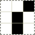
that we can represent with the following matrix
001
010
010
then we can map it into the 9-digit value 001010010
Back to MNIST dataset, where each image is a 28×28 pixel image, we will have an input composed by 784 binary digits.
The dataset can be therefore represented by a sequence of 70,000 rows, each one with 784 (input) + 10 (output) values
| Input (784 binary values) |
Output (10 binary values) |
| input#1 | 0010000000 |
| … | 0000000100 |
| input#70,000 | 1000000000 |
Out of these 70,000 items we will have then to take out a subset, e.g. 10,000 and use it for the Test dataset, leaving the other 60,000 for the Training set.
Whatever machine learning framework you adopt, almost certainly you’ll find MNIST among the first examples. It is considered so fundamental that you’ll find it packaged and organized to be used with just a few lines of code out-of-the-box.
This is for sure very handy since it just works, no hassles!
But there may be a flaw with this approach: you may not see clearly how the dataset is made of. In other words, you may have some difficulty when you decide to apply the same neural network used in MNIST to a similar, but different, use case. Let’s say for example you have a set of 50×50 images to be classified in 2 categories. How to proceed?
That’s why here we too will start from MNIST images, but we’ll see in detail how to transform them into a dataset.
Since we are practical and want to see some code running, we have to choose a framework to do that. We will do it with a great deep learning framework available for the Java language: Deeplearning4j!
As I wrote above, in order to get your first MNIST sample code running, you could just go to page
copy and run this Java code, but there are two key-lines
DataSetIterator mnistTrain = new MnistDataSetIterator(batchSize, true, rngSeed);
DataSetIterator mnistTest = new MnistDataSetIterator(batchSize, false, rngSeed);
which are too concise to understand how exactly the training and test datasets were built.
In this tutorial we will replace these with more detailed lines of code, so you can generalize from this example and experimenting with other datasets, maybe with your own images, which may not be 28×28 or maybe not event 0-9 digits!
In order to do so, we need to download the MNIST images dataset, but where can we find it?
Indeed you can download it from several sources and formats, but here we have a hint.
If you look at some other Java classes in the same GitHub repository, for example here:
in a comment, we read:
* Data is downloaded from
* wget http://github.com/myleott/mnist_png/raw/master/mnist_png.tar.gz
* followed by tar xzvf mnist_png.tar.gz
Ok, so let’s download
http://github.com/myleott/mnist_png/raw/master/mnist_png.tar.gz
and unzip somewhere, e.g. in /home/<user>/dl4j/ so to have the following situation
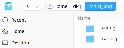 |
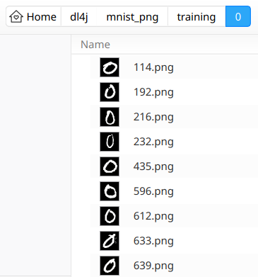
As you see, the dataset is split into two folders: training and testing, each one containing 10 subfolders, labeled 0 to 9, each one in turn containing thousands (almost 6,000) of image samples of handwritten digits correspondent to the label identified by the subfolder name.
So for instance the training/0 subfolder shows something like this
 |
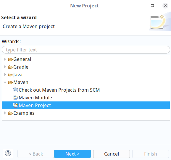
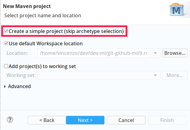
We are now ready to start working with Eclipse: let’s start it with a brand new workspace and create a new simple Maven Project (skip archetype selection)
 |
 |
 |
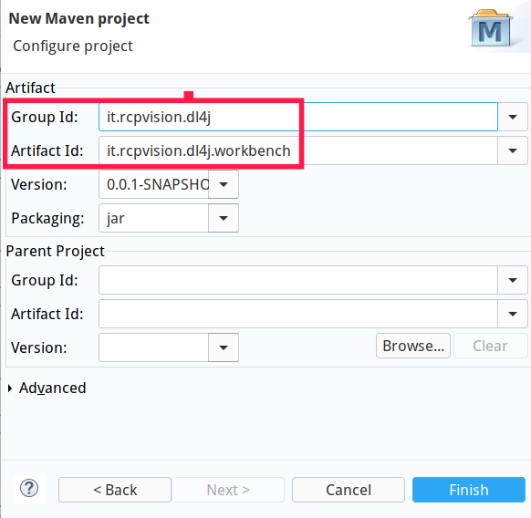
give it a Group Id and an Artifact Id, e.g. it.rcpvision.dl4j and it.rcpvision.dl4j.workbench
 |
Now open file pom.xml and add a dependency to deeplearning4j and other needed libraries
 	<dependencies>
		<dependency>
			<groupId>org.nd4j</groupId>
			<artifactId>nd4j-native-platform</artifactId>
			<version>1.0.0-beta4</version>
		</dependency>
		<dependency>
			<groupId>org.deeplearning4j</groupId>
			<artifactId>deeplearning4j-core</artifactId>
			<version>1.0.0-beta4</version>
		</dependency>
		<dependency>
			<groupId>org.slf4j</groupId>
			<artifactId>slf4j-jdk14</artifactId>
			<version>1.7.26</version>
		</dependency>
	</dependencies>
Then we can create a package called it.rcpvision.dl4j.workbench and a Java class named MnistStep1 with an empty main method.
In order to avoid doubts about imports of subsequent classes here are the needed imports
import java.io.File;
import java.io.IOException;
import java.util.Collections;
import java.util.List;
import java.util.Random;import org.datavec.image.loader.NativeImageLoader;
import org.deeplearning4j.datasets.iterator.impl.ListDataSetIterator;
import org.deeplearning4j.nn.conf.MultiLayerConfiguration;
import org.deeplearning4j.nn.conf.NeuralNetConfiguration;
import org.deeplearning4j.nn.conf.layers.DenseLayer;
import org.deeplearning4j.nn.conf.layers.OutputLayer;
import org.deeplearning4j.nn.multilayer.MultiLayerNetwork;
import org.deeplearning4j.nn.weights.WeightInit;
import org.deeplearning4j.optimize.listeners.ScoreIterationListener;
import org.nd4j.evaluation.classification.Evaluation;
import org.nd4j.linalg.activations.Activation;
import org.nd4j.linalg.api.ndarray.INDArray;
import org.nd4j.linalg.dataset.DataSet;
import org.nd4j.linalg.dataset.api.iterator.DataSetIterator;
import org.nd4j.linalg.dataset.api.preprocessor.ImagePreProcessingScaler;
import org.nd4j.linalg.factory.Nd4j;
import org.nd4j.linalg.learning.config.Nesterovs;
import org.nd4j.linalg.lossfunctions.LossFunctions.LossFunction;
import org.slf4j.Logger;
import org.slf4j.LoggerFactory;
Let’s define the constants we will use throughout the rest of the code:
//The absolute path of the folder containing MNIST training and testing subfolders
private static final String MNIST_DATASET_ROOT_FOLDER = "/home/vincenzo/dl4j/mnist_png/";
//Height and widht in pixel of each image
private static final int HEIGHT = 28;
private static final int WIDTH = 28;
//The total number of images into the training and testing set
private static final int N_SAMPLES_TRAINING = 60000;
private static final int N_SAMPLES_TESTING = 10000;
//The number of possible outcomes of the network for each input,
//correspondent to the 0..9 digit classification
private static final int N_OUTCOMES = 10;
Now, since we need to build two separate datasets (one for the training and another for the testing) that works in the same way and that only differ from the data they contain, it does make sense to create a reusable method for both.
So let’s define a method with the following signature:
private static DataSetIterator getDataSetIterator(String folderPath, int nSamples) throws IOException
where first parameter is the absolute path of the folder (training or testing) that contains the 0..9 subfolders with the samples, while the second is the total number of sample images included in the folder itself.
In this method we start by listing the 0..9 subfolders
File folder = new File(folderPath);
File[] digitFolders = folder.listFiles();
then we create two objects that will help us translating each image into a sequence of 0..1 input values
NativeImageLoader nil = new NativeImageLoader(HEIGHT, WIDTH);
ImagePreProcessingScaler scaler = new ImagePreProcessingScaler(0,1);
The first (NativeImageLoader) will be responsible to read the image pixels as a sequence of 0..255 integer values (where 0 is black and 255 is white – please note that each image has a white foreground and black background).
The second (ImagePreProcessingScaler) will scale each of the above values in a 0..1 (float) range, so that for instance every 255 integer value will become 1.
Then we need to prepare the arrays that will hold the input and output (remember: we are into a generic method that will handle both the training and testing set in the same way)
INDArray input = Nd4j.create(new int[]{ nSamples, HEIGHT*WIDTH });
INDArray output = Nd4j.create(new int[]{ nSamples, N_OUTCOMES });
In this way the input is a matrix with nSamples rows and 784 columns (the serialized 28×28 pixels of the image), while the output has the same number of rows (this dimension always matches between input and output), but 10 columns (the outcomes)
Now it’s time to scan each 0..9 folder and each image inside them, transform the image and the correspondent label (the digit it represents) into floating 0..1 values and populate the input and output matrixes.
int n = 0;
//scan all 0..9 digit subfolders
for (File digitFolder : digitFolders) {
  //take note of the digit in processing, since it will be used as a label
  int labelDigit = Integer.parseInt(digitFolder.getName());
  //scan all the images of the digit in processing
  File[] imageFiles = digitFolder.listFiles();
  for (File imageFile : imageFiles) {
    //read the image as a one dimensional array of 0..255 values
    INDArray img = nil.asRowVector(imageFile);
    //scale the 0..255 integer values into a 0..1 floating range
    //Note that the transform() method returns void, since it updates its input array
    scaler.transform(img);
    //copy the img array into the input matrix, in the next row
    input.putRow( n, img );
    //in the same row of the output matrix, fire (set to 1 value) the column correspondent to the label
    output.put( n, labelDigit, 1.0 );
    //row counter increment
    n++;
  }
}
Now, by composing the input and output matrixes, our method can build and return a DataSetIterator that the network can use
//Join input and output matrixes into a dataset
DataSet dataSet = new DataSet( input, output );
//Convert the dataset into a list
List<DataSet> listDataSet = dataSet.asList();
//Shuffle its content randomly
Collections.shuffle( listDataSet, new Random(System.currentTimeMillis()) );
//Set a batch size
int batchSize = 10;
//Build and return a dataset iterator that the network can use
DataSetIterator dsi = new ListDataSetIterator<DataSet>( listDataSet, batchSize );
return dsi;
With this method available we can now start using it into the main method in order to build the training dataset iterator.
long t0 = System.currentTimeMillis();
DataSetIterator dsi = getDataSetIterator(MNIST_DATASET_ROOT_FOLDER + "training", N_SAMPLES_TRAINING);
Now we can build the network, just as in the above mentioned deeplearning4j example on GitHub repository
int rngSeed = 123;
int nEpochs = 2; // Number of training epochs

log.info("Build model....");
MultiLayerConfiguration conf = new NeuralNetConfiguration.Builder()
  .seed(rngSeed) //include a random seed for reproducibility
  // use stochastic gradient descent as an optimization algorithm
  .updater(new Nesterovs(0.006, 0.9))
  .l2(1e-4)
  .list()
  .layer(new DenseLayer.Builder() //create the first, input layer with xavier initialization
    .nIn(HEIGHT*WIDTH)
    .nOut(1000)
    .activation(Activation.RELU)
    .weightInit(WeightInit.XAVIER)
    .build())
  .layer(new OutputLayer.Builder(LossFunction.NEGATIVELOGLIKELIHOOD) //create hidden layer
    .nIn(1000)
    .nOut(N_OUTCOMES)
    .activation(Activation.SOFTMAX)
    .weightInit(WeightInit.XAVIER)
    .build())
  .build();
Here we have a simple fully connected network with one hidden layer containing 1000 nodes.
Then the network can be trained using our brand new training dataset iterator (dsi)
MultiLayerNetwork model = new MultiLayerNetwork(conf);
model.init();
//print the score with every 500 iteration
model.setListeners(new ScoreIterationListener(500));
log.info("Train model....");
model.fit(dsi, nEpochs);
After this phase (that may take a quite a while) we can reuse our method to build the testing set iterator and evaluate this set while printing some statistics about how now the network performs over the testing set.
DataSetIterator testDsi = getDataSetIterator( MNIST_DATASET_ROOT_FOLDER + "testing", N_SAMPLES_TESTING);
log.info("Evaluate model....");
Evaluation eval = model.evaluate(testDsi);
log.info(eval.stats());

long t1 = System.currentTimeMillis();
double t = (double)(t1 - t0) / 1000.0;
log.info("\n\nTotal time: "+t+" seconds");
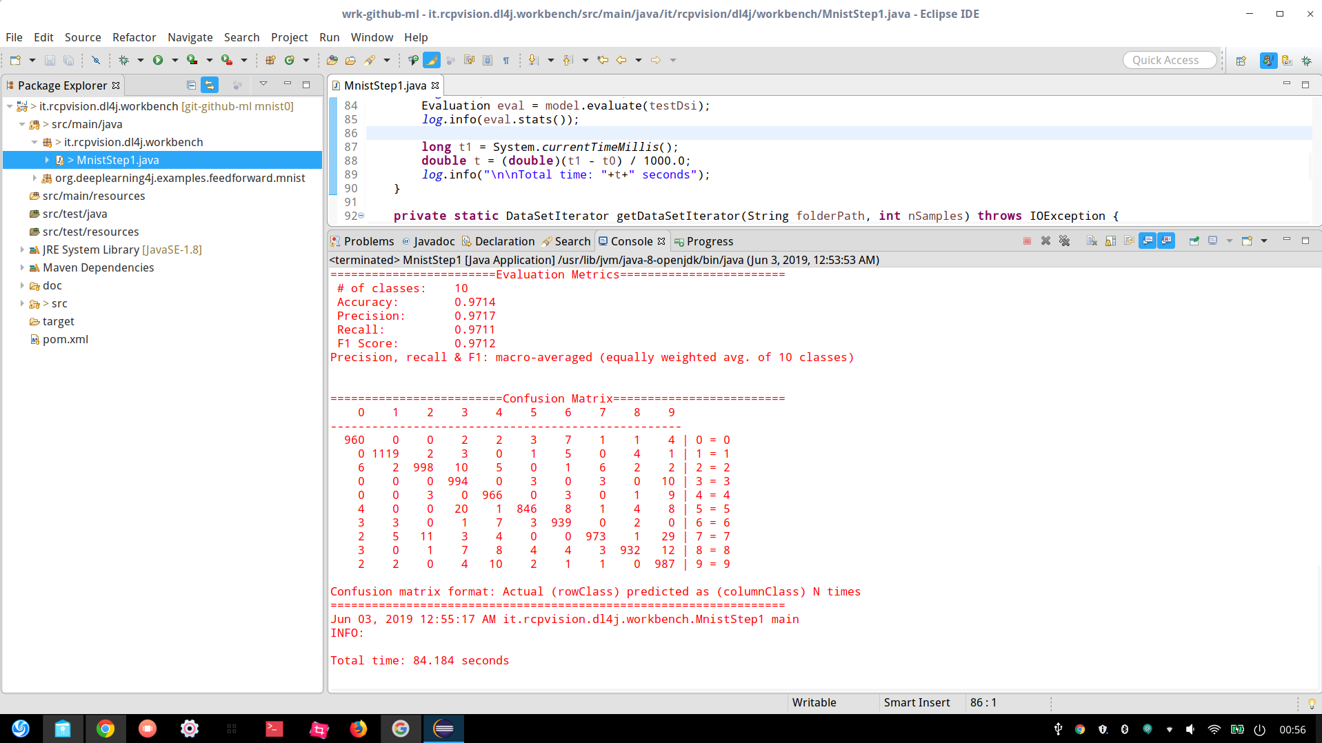
As we can see in the following image, we can reach an accuracy of 97% even with an extremely simple network.
Less than one and a half minute for a complete training and testing phase (all included); not bad, isn’t it?
 |
Next > Convolutional Neural Networks with Eclipse Deeplearning4j

This was absolutely the best starter guide i could find on DeepLearning4J. Took me 10 mins to get everything setup and i understood what i was doing.
its really great
[…] published on rcp-vision.com. Reproduced here with consent of the original author: Vincenzo Caselli, who describes himself like […]
GREAT!